ComputerGraphics
12. コンピュータグラフィックス
12.1. 概要
コンピュータ・グラフィックス(CG)はゲーム,映画や,画像などからよく知られているものです.CGを作成するための驚くべきソフトウェアが利用可能ですが,それらはどの様に動作しているのでしょうか?コンピュータ科学の専門家の役割には,ただ単にグラフィック・ソフトを使うだけではなく,そのようなシステムの開発や新しい技術を発明することが求められています.
娯楽産業は常に新しいグラフィック・ソフトを開発しようとしています.それによって私たちは,今までにできなかったことの限界を超えたり,新しい体験をしたりすることができるのです.この事は,単純な2次元映画から,詳細にわたる3次元イメージを使いコンピュータで生成されたリアリティのあるアニメ映画への進化の過程を見ることで理解できると思います.
映画やゲームの制作会社は次の大作をつくるために,いつも既存のソフトウェアを使うわけではありません.今までに見たこともないような新しい作品を作るために,より良いグラフィック技術を生み出すために,制作会社はコンピュータ科学者を必要としています.創造性の可能性には限りがないのです!
CGは幅広くいろいろな場面で使われています.例えば,ゲームやアニメ映画は誰でもよく知っているでしょう.しかし,大量のデータ(例えば1日に行われるすべての携帯電話の通話状況など)を視覚化するのにも,グラフィック技術は用いられているのです.例えば仮想現実(VR,バーチャル・リアリティ)や拡張現実(AR)の世界を作るなどして表示したり,グラフィカル・ユーザ・インタフェースをアニメーション化したりします.
Jargon Buster: Pixels
A digital image on a screen or printer is physically made up of a grid of tiny squares called pixels. They are usually too small to see easily (otherwise the image would look blocky). Photographs usually use millions of pixels (a megapixel is a million pixels; for example, a screen that is 1080 pixels across and 720 down would contain 777,600 pixels, or 0.7776 megapixels).
The pixels is fundamental to computer graphics, as a lot of the work of computer graphics programmers is taking some abstract idea (such as objects in a scene), and working out the colour each pixel should be to make the viewer think they are looking at the scene. A digital camera also does this - but it just senses the colour falling on each of its millions of sensors, and stores those so that the pixels can be displayed when needed.
この章では,CGを作成する上で用いられている基本的な技術のいくつかを見ていきます.これらはグラフィック・プログラミングで使われている技術的なアイデアを私たちに与えてくれるでしょう.しかしこれはまた,可能性の正に始まりに過ぎないのです.
この章では,ブラウザー上で,3次元グラフィックを描画することができるWebGLというシステムを使います.もしブラウザーが正しくセットアップされているならば,画面の右側にティポットを見ることができます.また,ボタンをクリックするとティポットを回転させることができます.もし動かないとか処理速度が遅いという場合は,どうすれば動くかといった情報についてはここ(←リンクあり)を見てください.
12.2. グラフィックスの変形
CG画像は単に膨大な数学的な計算の結果に過ぎません.実際,典型的な画像は数百万ピクセル(画素)くらいで構成されていますが,そのあらゆるピクセルの一つ一つを何色にすべきという大量の計算結果が含まれているのです.
それでは,グラフィックス・プログラミングで必要とされる計算で,単純ではあるものの一般的な計算から始めてみましょう.次のウィジェットにはそれぞれの表面が描かれた立方体の画像があります.そこで,変換と呼ばれる操作を用いて立方体を動かして見ましょう.ただし,立方体が置かれている位置(x, y, z)だけを指定することができます.
このウィジェットでは,3方向にしか移動できない変形を試すことができます.移動できる方向はx(左右),y(上下)とz(前後)です.それぞれの移動には「移動」に数字を入力します.反対方向に移動したい場合はマイナスの値にします.立方体の三つの面には絵文字が描かれていますので,立方体を移動させることで見つけてください.それらの絵文字を「暗号」と書かれた回転体を回して,描かれていた絵文字を揃えてください.ただし,絵文字の順番は問いません.最後に「謎を解く」のボタンを押したらゴールとなります.
★コンテンツは準備中です★
ここでは,立方体に3次元の方向に平行移動を行う変形を試してみたことになります.平行移動とは,左右,上下,前後という3次元の動きを意味しています.
他の一般的な変形として回転があります.次のウィジェットでは立方体を回転させ,側面に描かれている絵文字を探しましょう(回転は角度で指定します).
★コンテンツは準備中です★
CGで使われる変形にはいくつかの種類があります.しかし、最も一般的なものは平行移動(物を動かす),回転(回す)そしてスケーリング(サイズを変える)です.それらは物に対する変形だけでなく,カメラや光源の位置などの変形もグラフィックスではよく利用されています.
ここでは,いろいろな画像に変形を行うことができます.まず手作業で一度に一つずつ変化させることから始めます.ただし,この作業をするために速いショートカットな方法である行列を使います.まず,3次元で考えるよりは少し易しい2次元でこれらの作業を見ていくことにします.
次のウィジェットには矢印が描かれています.そして,その右側にはその矢印を構成する7つの頂点の座標が表示されています.矢印は,中心を0とした直交座標(デカルト座標と呼ばれる)系の格子上の点にあります.点はxとyの二つの数字で表現され,通常は(x, y)の様に書かれます.xの値は中心点から右方向にどのくらい離れているかを示し,yの値は中心点から上方向にどのくらい離れているかを示しています.例えば,示されている座標の1番目は矢印の先端で(0, 2)となっていますが,これは中心から右に0(つまり中心と同じ位置),上に二つ目の位置にあるということになります.では,1番下の座標である(2, 0)は矢印のどの部分になるでしょうか?また,xの値がマイナスの場合はどの様な意味があるのでしょうか?
上の方にある座標のリストは矢印の最初の位置を示すためにあります.そして,下の方のリストには,値を入力することで矢印の頂点を移動させることができ変形を行います.最初からある矢印は緑で,そして動かしたものは青で描画されます.
★コンテンツは準備中です★
それではまず,すべての点のxの値に2を加え,yの値すべてに3を加えてみましょう.下の表には,計算した後の値を入力しても良いですし,たとえば「0.5+2」の様に計算式を入力しても大丈夫です.その結果,最初の矢印にどの様な効果を与えたでしょうか?ここで,負の数を加える場合は正しく計算をするように注意しましょう.たとえば,-0.5に2を加えると1.5になります.次に,すべての座標の値からそれぞれ3を引いたらどうなるでしょうか?
上記の変形は平行移動(矢印を格子の周りで平行移動させている)と呼ばれています.この種の変形はグラフィックスではシーンのどこに物体を置くかを決める際に利用されます.しかし,他にもいろいろな利用法があります.たとえば物体を経路に沿って動かして動画を作成する場合や,仮想カメラ(又は視点)の位置を決める場合などです.
次のウィジェットでは,下の座標表すべてに上の表の値を2倍にしてみてください.この変形の効果はどうなるのでしょうか?2倍ではなく10倍だとどうでしょうか?または,0.5倍では?xの値だけにかけ算をしたらどうなるでしょうか?
★コンテンツは準備中です★
この変形はスケーリングと呼ばれています.そして物体のサイズを制御するのに使われています.たとえば,物体が近くや遠くにあるように見せるなどの視覚効果を得るために使われています.
次のウィジェットで,青い矢印を赤い矢印に一致させるようにしてみてください.ここでは,平行移動とスケーリングの両方を利用しないといけません.
★コンテンツは準備中です★
次に,それぞれの座標で,xとyの値を入れ替えたらどうなるでしょうか?
★コンテンツは準備中です★
これは簡単な回転変形となっています.これはある場面での物体の位置決めやカメラアングルなどの場所決めなどに利用されています.
Typing all these coordinates by hand is inefficent. Luckily there's a much better way of achieving all this. Read on!
12.2.1.行列変形
それぞれの座標の値を別々に変えるよりも,変形を決めるもっと簡単な方法があります.グラフィックスでは通常,変形は行列計算によって行われます.行列計算は座標をいちいち計算するよりも簡単な計算をすることで,短い表記にすることができます.2次元変形のための行列は4つの値をもっています.2次元スケーリングで,xとyのそれぞれの値を2倍するための行列は次のように書きます:
[2 0
0 2]
以下のウィジェットでこの行列を入力してみて,何が起こるかを見てみましょう(「行列乗算」の「1」のところを「2」に変えてみましょう).上の行の左側の数字はすべてのxの値を2倍するという意味で,下の行の右側の数字はすべてのyの値を2倍するという意味です.とりあえず,他の値は0としておきます.
★コンテンツは準備中です★
(ここでは,ウィジェットを別のウィンドウで開いて,以下の文中の数値を見ながら使いたいと思うかもしれませんね.)
[3003]
それで,行列を
[30
03]
に変えたらどうなるでしょうか?
or
[0.2000.2]
また,
[0.2 0
0 0.2]
ではどうでしょうか?
ウィジェットの中で,「変換の追加」の値はすべてのxとyの座標に値を加えます.どうなるか試してみてください.では,赤色の矢印に一致するような行列の値を見つけてみましょう.
[2004]
次の行列を使うと何が起こるでしょうか?
[2 0
0 4]
[0110]
では,次の行列を試してみましょう:
[0 1
1 0]
この行列は矢印を右に回転させます.
[2004]
行列の簡単な見方としては,上の行は変形後のxの値を決めます.つまり変形前のxとyの値が新しいxの値にどのくらい寄与するかを示しています.そこで行列
[2 0
0 4]
では,
上の行は,変形後のxの値は,変形前のxの値を2倍してyの値を何もしない,つまりすべてのxの値を2倍することを意味しています.2行目は変形後のyの値を決定します.上の行列の例では,変形後のyには変形前のxの値は使用せずに,yの値を4倍するという意味になります.つまり,この行列を使うとすべてのxの位置は2倍された値となり,yの位置は4倍された値となるのです.
[0 1
1 0]
の行列について説明しましょう.変形後のxの値は変形前のxの影響を全く受けません.しかし,変形前のyの値そのものが変形後のxの値となります.そして逆(変形後のyの値)も同様です.これはすべてのxとyの値を入れ替えており,これは右への回転と同じ働きをします.
面白い変形としては,次の
[0.7 -0.7
0.7 0.7]
といった行列の様に,小さな値を使う時です.
この行列を使うと,変形後のx座標は変形前のxの値の0.7倍と変形前のyの値の0.7倍を足し合わせた物となります.
一般的に回転する角度が与えられている場合の画像の回転には三角関数のサイン(sin),コサイン(cos)を使用します.画像を角度θ度だけ回転するには,次の値を持った行列が必要となります.
[cos(θ) sin(θ)
−sin(θ) cos(θ)]
これらの計算もまたウィジェットで直接計算させることができます.もし,cos(60)と入力したらコサイン60度の値(0.5になります)を計算してくれます.または,サインやコサインの計算結果の値を直接入力することもできます.例えば,上記の行列にあった0.7はsin(45)とほぼ同じとなります(正確にはsin(45)は√(0.5)なので0.70710678...となりますが,今回の例としては0.7で十分です).
★コンテンツは準備中です★
では,360度回転させるときの行列はどの様なものでしょうか?
スケーリングに使う時の一般的な行列は,ちょっとだけ簡単です.例えばs倍したいのであれば次の行列を使えばよいのです.
[s 0
0 s]
平行移動はこの種の行列によって表現することはできません.しかし,今回提供しているウィジェットでは,平行移動のためのxとyの値を入力するための場所が用意されています
元の矢印を平行移動させて赤い矢印に合わせてみましょう.
★コンテンツは準備中です★
では、元の矢印を次のようにスケーリングさせて,そして平行移動させて赤い矢印に合わせてみましょう.
★コンテンツは準備中です★
次のウィジェットは平行移動をしてからスケーリングを行います.このウィジェットを使って青い矢印を赤い矢印に変形してみましょう.操作の順番が違うと異なった結果になってしまいますね!
★コンテンツは準備中です★
上の例では,スケーリングは物体がどのくらい座標の中心から離れているかによって影響されることに気づくと思います.もし,物体が置かれている場所(座標の中心にいない場合)を中心にスケーリングしたい場合,簡単な方法は一旦座標の中心に平行移動させてからスケーリングをして,そして元の場所に平行移動させることです.次のウィジェットは矢印を移動,スケーリング,移動(元の場所に)させることができます.
矢印の先端は(-8, 7)にあるので,まず(0, 0)に移動して,次に2倍して,そして(-8, 7)に移動させなければいけません.
★コンテンツは準備中です★
同様な問題は回転されるときにも生じます.
それでは矢印を45度回転させてみましょう.先端を一旦原点に移動して,回転させ,そして元の位置に移動して戻す必要があります.
★コンテンツは準備中です★
以下の2つの例は,回転,スケーリング,そして回転移動を組み合わせて使います.赤の矢印に合わせるために,2つまでの行列と平行移動を使うことができます.このとき,一つ目の行列の計算結果が二つ目の行列への入力値となります.おっと!矢印の太さが2倍になっていますが高さは同じになっていますよ!
それでは,青い矢印を二つの行列(一つはスケーリング,もう一つは回転に使います)と平行移動を使って赤い矢印に合わせましょう.
★コンテンツは準備中です★
次のウィジェットでも三つの操作を使わなければなりません.
★コンテンツは準備中です★
これらの組み合わせによる変形は一般的なことです.そして物体のすべての点に対してそれぞれの行列計算を行わなければならないため,非常に手間がかかるように見えます.今回の矢印はたった七つの点で構成されていましたが,複雑な画像になれば数千から数百万の点で構成されています.しかし幸いにも,すべての行列操作を事前に一つにまとめて,各点への適用時にはたった一つの行列操作で行うことで計算ができるのです.
12.2.2. 変形の結合
同じ画像に適用されるいくつかの変形は,すべての変形効果を結合して一つの行列を作ることでより効率よくすることができます.すべての行列をかけ算することで行列の結合をすることができます.
二つの行列をかけ算するのは.それぞれの行列の対応する要素をかけ算すれば良いわけではありません.aとbという行列のかけ算は以下のように計算します.
[a11 a12
a21 a22]
☓
[b11 b12
b21 b22]
=
[a11☓b11+a21☓b12 a12☓b11+a22☓b12
a11☓b21+a21☓b22 a12☓b21+a22☓b22]
これは多少面倒くさく見えるかもしれませんが,この計算は一回だけ行えばよく,変形を1回の操作で完了することができる行列を得ることができるのです.
簡単な例題でみてみましょう.2倍にスケーリングして45度回転をすることを考えます.二つの行列のかけ算は次のように計算されます.
[2 0
0 2]
☓
[0.7 −0.7
0.7 0.7]
=
[2×0.7+0×−0.7 0×0.7+2×−0.7
2×0.7+0×0.7 0×0.7+2×0.7]
=
[1.4 −1.4
1.4 1.4]
最後の行列の値をウィジェットに入力し,2倍にスケーリングされ45度回転しているかどうかを確かめてみてください.
★コンテンツは準備中です★
それでは,自分で作った変形のための二つの行列のかけ算をして,それが期待される結果を出しているかどうかをみてみましょう.
★コンテンツは準備中です★
コンピュータ・グラフィックス・システムでは,多くの変形を結合することができます.そして,それは一度に二つずつの行列をかけ算しながら最終的にはすべての行列を一つの行列で変形できるようにまとめることができるのです.この変形は何百万もの点に適用することができ,その計算にかかる時間を短縮することに成果を上げることができるのです.
続く節では,行列のかけ算を計算してくれるウィジェットが用意されており,行列の結合を調べるきっかけを提供しています.
12.2.3. 3次元の変形
これまでは,私たちは2次元の変形をおこなってきました.これを3次元で行うために,画面での深さを表すz軸が必要となります.3次元で表される点を操作する行列は3行3列になります.例えば,物体のサイズを2倍する3次元行列は,次のようにそれぞれのx,y,zの値を2倍します.
[2 0 0
0 2 0
0 0 2]
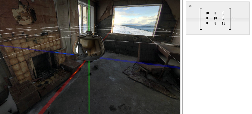
以下のウィジェットで,画像のスケールを変えてみてください(最初は,x,y,zすべての3次元方向に10倍するようになっています).
★コンテンツは準備中です★
The above image mesh has 3644 points in it, and your matrix was applied to each one of them to work out the new image.
Translation requires 3 values, which are added to the *x*, *y* and *z* coordinates of each point in an object.
上のウィジェットでの画像には3644個の点が使われています.従って指定した行列はすべての点に適用されて,新しい画像が描かれるのです.また,平行移動は物体のすべての点に対して,x,y,z座標に加えるべき3つの値を必要とします.
In the following interactive, try moving the teapot left and right ( x ), up and down ( y ), and in and out of the screen ( z ) by adding a “vector” to the operations. Then try combining all three.
それでは次のウィジェットで,ティポットを「+ベクトル」の機能を使ってそれぞれ左右(x方向),上下(y方向),そして前後(z)に移動させてみましょう.そして,xyzの移動を一つの行列に結合しましょう.
★コンテンツは準備中です★
Rotation is trickier because you can now rotate in different directions. In 2D rotations were around the centre (origin) of the grid, but in 3D rotations are around a line (either the horizontal x-axis, the vertical y-axis, or the z-axis, which goes into the screen!)
回転は,いままでとは異なる方向にも回転するため,より慎重に行う必要があります.2次元での回転では,私たちはグリッドの原点を中心に回転させました.しかし,3次元の回転では,線(水平線であるx軸,垂直線であるy軸,前後への線であるz軸)の周りに回転を行います.
The rotation we used earlier can be applied to 3 dimensions using this matrix:
⎡⎣⎢⎢cos(θ)sin(θ)0−sin(θ)cos(θ)0001⎤⎦⎥⎥
Try applying that to the image above. This is rotating around the z-axis (a line going into the screen); that is, it’s just moving the image around in the 2D plane. It’s really the same as the rotation we used previously, as the last line (0, 0, 1) just keeps the z point the same.
Try the following matrix, which rotates around the x-axis (notice that the x value always stays the same because of the 1,0,0 in the first line):
⎡⎣⎢⎢1000cos(θ)sin(θ)0−sin(θ)cos(θ)⎤⎦⎥⎥
And this one for the y-axis:
⎡⎣⎢⎢cos(θ)0−sin(θ)010sin(θ)0cos(θ)⎤⎦⎥⎥
The following interactive allows you to combine 3D matrices.
You can experiment with moving the teapot around in space, changing its size, and angle.
Think about the order in which you need to combine the transforms to get a particular image that you want.
For example, if you translate an image and then scale it, you’ll get a different effect to scaling it then translating it. If you want to rotate or scale around a particular point, you can do this in three steps (as with the 2D case above): (1) translate the object so that the point you want to scale or rotate around is the origin (where the x, y and z axes meet), (2) do the scaling/rotation, (3) translate the object back to where it was. If you just scale an object where it is, its distance from the origin will also be scaled up.
★コンテンツは準備中です★
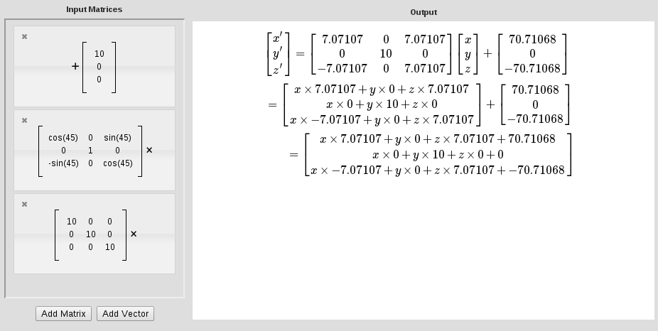
In the above examples, when you have several matrices being applied to every point in the image, a lot of time can be saved by converting the series of matrices and transforms to just one formula that does all of the transforms in one go. The following interactive can do those calculations for you.
For example, in the following interactive, type in the matrix for doubling the size of an object (put the number 2 instead of 1 on the main diagonal values), then add another matrix that triples the size of the image (3 on the main diagonal). The interactive shows a matrix on the right that combines the two — does it look right?
Multiple transforms
★コンテンツは準備中です★
The interactive also allows you to combine in translations (just three numbers, for x, y and z). Try combining a scaling followed by a translation. What if you add a rotation — does the order matter?
In case you’re wondering, the interactive is using the following formula to combine two matrices (you don’t have to understand this to use it). It is called matrix multiplication, and while it might be a bit tricky, it’s very useful in computer graphics because it reduces all the transformations you need to just one matrix, which is then applied to every point being transformed. This is way better than having to run all the matrices of every point.
12.2.4. Project: 3D transforms
For this project, you will demonstrate what you’ve learned in the section above by explaining a 3D transformation of a few objects. You should take screenshots of each step to illustrate the process for your report.
The following scene-creation interactive allows you to choose objects (and their colours etc.), and apply one transformation to them. To position them more interestingly, you will need to come up with multiple transformations (e.g. scale, then rotate, then translate), and use the “simplifier” interactive to combine all the matrices into one operation.
The scene-creation interactive can be run from here:
To generate combined transformations, you can use the following transform simplifier interactive:
Because you can’t save your work in the interactives, keep notes and screen shots as you go along. These will be useful for your report, and also can be used if you need to start over again.
Introduce your project with a examples of 3D images, and how they are used (perhaps from movies or scenes that other people have created). Describe any innovations in the particular image (e.g. computer generated movies usually push the boundaries of what was previously possible, so discuss what boundaries were moved by a particular movie, and who wrote the programs to achieve the new effects).
For your project, try putting a few objects in a particular arrangement (e.g. with the teapot sitting beside some cups), and explain the transforms needed to achieve this, showing the matrices needed.
Give simple examples of translation, scaling and rotation using your scene.
You should include multiple transforms applied to one object, and show how they can be used to position an object.
Show how the matrices for a series of transforms can be multiplied together to get one matrix that applies all the transforms at once.
Discuss how the single matrix derived from all the others is more efficient, using your scene as an example to explain this.
12.3. Drawing lines and circles
A fundamental operation is computer graphics is to draw lines and circles. For example, these are used as the components of scalable fonts and vector graphics; the letter “i” is specified as a series of lines and curves, so that when you zoom in on it the computer can redraw it at whatever resolution is needed.

In 3D graphics shapes are often stored using lines and curves that mark out the edges of flat surfaces, each of which is so small that you can’t see them unless you zoom right in.

The lines and circles that specify an object are usually given using numbers (for example, a line between a given starting and finishing position or a circle with a given centre and radius). From this a graphics program must calculate which pixels on the screen should be coloured in to represent the line or circle.
For example, here’s a grid of pixels with 5 lines shown magnified. The vertical line would have been specified as going from pixel (2,9) to (2,16) — that is, starting 2 across and 9 up, and finishing 2 across and 16 up. Of course, this is only a small part of a screen, as normally they are more like 1000 by 1000 pixels or more; even a smartphone can be hundreds of pixels high and wide.

These are things that are easy to do with pencil and paper using a ruler and compass, but on a computer the calculations need to be done for every pixel, and if you use the wrong method then it will take too long and the image will be displayed slowly or a live animation will appear jerky. In this section we will look into some very simple but clever algorithms that enable a computer to do these calculations very quickly.
12.3.1. Line drawing
To draw a line, a computer must work out which pixels need to be filled so that the line looks straight. You can try this by colouring in squares on a grid, such as the one below (they are many times bigger than the pixels on a normal printer or screen). We’ll identify the pixels on the grid using two values, (x,y), where x is the distance across from the left, and y is the distance up from the bottom. The bottom left pixel below is (0,0), and the top right one is (19,19).
On the following grid, try to draw these straight lines by filling in pixels in the grid:
- from (2, 17) to (10, 17)
- from (18, 2) to (18, 14)
- from (1, 5) to (8, 12)

Drawing a horizontal, vertical or diagonal line like the ones above is easy; it’s the ones at different angles that require some calculation.
Without using a ruler, can you draw a straight line from A to B on the following grid by colouring in pixels?

Once you have finished drawing your line, try checking it with a ruler. Place the ruler so that it goes from the centre of A to the centre of B. Does it cross all of the pixels that you have coloured?
12.3.2. Using a formula to draw a line
The mathematical formula for a line is y = mx + b. This gives you the y value for each x value across the screen, where m is the slope of the line and b is where it crosses the y axis. In other words, for x pixels across, the pixel to colour in would be (x, mx + b).
For example, choosing m=2 and b=3 means that the line would go through the points (0,3), (1,5), (2,7), (3,9) and so on. This line goes up 2 pixels for every one across (m=2), and crosses the y axis 3 pixels up (b=3).
You should experiment with drawing graphs for various values of m and b (for example, start with b=0, and try these three lines: m=1, m=0.5 and m=0) by putting in the values. What angle are these lines at?
The mx + b formula can be used to work out which pixels should be coloured in for a line that goes between (x_1,y_1) and (x_2,y_2). What are (x_1,y_1) and (x_2,y_2) for the points A and B on the grid below?
See if you can work out the m and b values for a line from A to B, or you can calculate them using the following formulas:
m &= \frac{(y_2 - y_1)}{(x_2 - x_1)}\\ b &= \frac{(y_1x_2 - y_2x_1)}{(x_2-x_1)}\\
Now draw the same line as in the previous section (between A and B) using the formula y = mx + b to calculate y for each value of x from x_1 to x_2 (you will need to round y to the nearest integer to work out which pixel to colour in). If the formulas have been applied correctly, the y value should range from y_1 to y_2.
Once you have completed the line, check it with a ruler. How does it compare to your first attempt?
Now consider the number of calculations that are needed to work out each point. It won’t seem like many, but remember that a computer might be calculating hundreds of points on thousands of lines in a complicated image. In the next section we will explore a method that greatly speeds this up.
12.3.3. Bresenham’s Line Algorithm
A faster way for a computer to calculate which pixels to colour in is to use Brensenham’s Line Algorithm. It follows these simple rules. First, calculate these three values:
A &= 2 \times (y_2 - y_1) \\ B &= A - 2 \times (x_2 - x_1) \\ P & = A - (x_2 - x_1) \\
To draw the line, fill the starting pixel, and then for every position along the x axis:
- if P is less than 0, draw the new pixel on the same line as the last pixel, and add A to P.
- if P was 0 or greater, draw the new pixel one line higher than the last pixel, and add B to P.
- repeat this decision until we reach the end of the line.
Without using a ruler, use Bresenham’s Line Algorithm to draw a straight line from A to B:
Grid for drawing line from A to B
Once you have completed the line, check it with a ruler. How does it compare to the previous attempts?
12.3.4. Lines at other angles
So far the version of Bresenham’s line drawing algorithm that you have used only works for lines that have a gradient (slope) between 0 and 1 (that is, from horizontal to 45 degrees). To make this algorithm more general, so that it can be used to draw any line, some additional rules are needed:
- If a line is sloping downward instead of sloping upward, then when P is 0 or greater, draw the next column’s pixel one row below the previous pixel, instead of above it.
- If the change in Y value is greater than the change in X value, then the calculations for A, B, and the initial value for P will need to be changed. When calculating A, B, and the initial P, use X where you previously would have used Y, and vice versa. When drawing pixels, instead of going across every column in the X axis, go through every row in the Y axis, drawing one pixel per row.
In the grid above, choose two points of your own that are unique to you. Don’t choose points that will give horizontal, vertical or diagonal lines!
Now use Bresenham’s algorithm to draw the line. Check that it gives the same points as you would have chosen using a ruler, or using the formula y = mx+b. How many arithmetic calculations (multiplications and additions) were needed for Bresenhams algorithm? How many would have been needed if you used the y = mx+b formula? Which is faster (bear in mind that adding is a lot faster than multiplying for most computers).
You could write a program or design a spreadsheet to do these calculations for you — that’s what graphics programmers have to do.
12.3.5. Circles
As well as straight lines, another common shape that computers often need to draw are circles. An algorithm similar to Bresenham’s line drawing algorithm, called the Midpoint Circle Algorithm, has been developed for drawing a circle efficiently.
A circle is defined by a centre point, and a radius. Points on a circle are all the radius distance from the centre of the circle.

Try to draw a circle by hand by filling in pixels (without using a ruler or compass). Note how difficult it is to make the circle look round.
It is possible to draw the circle using a formula based on Pythagoras’ theorem, but it requires calculating a square root for each pixel, which is very slow. The following algorithm is much faster, and only involves simple arithmetic so it runs quickly on a computer.
12.3.6 Bresenham’s Midpoint Circle Algorithm
Here are the rules for the Midpoint Circle Algorithm for a circle around (c_{x}, c_{y}) with a radius of R:
E &= -R \\ X &= R \\ Y &= 0 \\
Repeat the following rules in order until Y becomes greater than X:
- Fill the pixel at coordinate (c_{x} + X, c_{y} + Y)
- Increase E by 2 \times Y + 1
- Increase Y by 1
- If E is greater than or equal to 0, subtract (2X - 1) from E, and then subtract 1 from X.
Follow the rules to draw a circle on the grid, using (c_{x}, c_{y}) as the centre of the circle, and R the radius. Notice that it will only draw the start of the circle and then it stops because Y is greater than X!
When y becomes greater than x, one eighth (an octant) of the circle is drawn. The remainder of the circle can be drawn by reflecting the octant that you already have (you can think of this as repeating the pattern of steps you just did in reverse). Reflect pixels along the X and Y axis, such that the line of reflection crosses the middle of the centre pixel of the circle. Half of the circle is now drawn, the left and the right half. To add the remainder of the circle, another line of reflection must be used. Can you work out which line of reflection is needed to complete the circle?
Jargon Buster : Quadrants and octants
A quadrant is a quarter of an area; the four quadrants that cover the whole area are marked off by a vertical and horizontal line that cross. An octant is one eighth of an area, and the 8 octants are marked off by 4 lines that intersect at one point (vertical, horizontal, and two diagonal lines).
To complete the circle, you need to reflect along the diagonal. The line of reflection should have a gradient of 1 or -1, and should cross through the middle of the centre pixel of the circle.
While using a line of reflection on the octant is easier for a human to understand, a computer can draw all of the reflected points at the same time it draws a point in the first octant because when it is drawing pixel with an offset of (x,y) from the centre of the circle, it can also draw the pixels with offsets (x,-y), (-x,y), (-x,-y), (y,x), (y,-x), (-y,x) and (-y,-x), which give all eight reflections of the original point!
By the way, this kind of algorithm can be adapted to draw ellipses, but it has to draw a whole quadrant because you don’t have octant symmetry in an ellipse.
12.3.7. Practical applications
Computers need to draw lines, circles and ellipses for a wide variety of tasks, from game graphics to lines in an architect’s drawing, and even a tiny circle for the dot on the top of the letter ‘i’ in a word processor. By combining line and circle drawing with techniques like ‘filling’ and ‘antialiasing’, computers can draw smooth, clear images that are resolution independent. When an image on a computer is described as an outline with fill colours it is called vector graphics — these can be re-drawn at any resolution. This means that with a vector image, zooming in to the image will not cause the pixelation seen when zooming in to bitmap graphics, which only store the pixels and therefore make the pixels larger when you zoom in. However, with vector graphics the pixels are recalculated every time the image is redrawn, and that’s why it’s important to use a fast algorithm like the one above to draw the images.
Outline fonts are one of the most common uses for vector graphics as they allow the text size to be increased to very large sizes, with no loss of quality to the letter shapes.
Computer scientists have found fast algorithms for drawing other shapes too, which means that the image appears quickly and it can be done on relatively slow hardware - for example, a smartphone needs to do these calculations all the time to display images, and reducing the amount of calculations can extend its battery life, as well as make it appear faster.
As usual, things aren’t quite as simple as shown here. For example, consider a horizontal line that goes from (0,0) to (10,0), which has 11 pixels. Now compare it with a 45 degree line that goes from (0,0) to (10,10). It still has 11 pixels, but the line is longer (about 41% longer to be precise). This means that the line would appear thinner or fainter on a screen, and extra work needs to be done (mainly anti-aliasing) to make the line look ok. We’ve only just begun to explore how techniques in graphics are needed to quickly render high quality images.
Project: Line and circle drawing
To compare Bresenham's method with using the equation of a line (y=mx+by=mx+b), choose your own start and end point of a line (of course, make sure it's at an interesting angle), and show the calculations that would be made by each method. Count up the number of additions, subtractions, multiplications and divisions that are made in each case to make the comparison. Note that addition and subtraction is usually a lot faster than multiplication and division on a computer.
You can estimate how long each operation takes on your computer by running a program that does thousands of each operation, and timing how long it takes for each. From this you can estimate the total time taken by each of the two methods. A good measurement for these is how many lines (of your chosen length) your computer could calculate per second.
If you're evaluating how fast circle drawing is, you can compare the number of addition and multiplication operations with those required by the Pythagoras formula that is a basis for the simple equation of a circle (for this calculation, the line from the centre of the circle to a particular pixel on the edge is the hypotenuse of a triangle, and the other two sides are a horizontal line from the centre, and a vertical line up to the point that we're wanting to locate. You'll need to calculate the y value for each x value; the length of the hypotenuse is always equal to the radius).
12.4. The whole story!
We've only scraped the surface of the field of computer graphics. Computer scientists have developed algorithms for many areas of graphics, including:
lighting (so that virtual lights can be added to the scene, which then creates shading and depth)
texture mapping (to simulate realistic materials like grass, skin, wood, water, and so on),
anti-aliasing (to avoid jaggie edges and strange artifacts when images are rendered digitally)
projection (working out how to map the 3D objects in a scene onto a 2D screen that the viewer is using),
hidden object removal (working out which parts of an image can't be seen by the viewer),
photo-realistic rendering (making the image as realistic as possible), as well as deliberately un-realistic simulations, such as "painterly rendering" (making an image look like it was done with brush strokes), and
efficiently simulating real-world phenomena like fire, waves, human movement, and so on.
The matrix multiplication system used in this chapter is a simplified version of the one used by production systems, which are based on homogeneous coordinates. A homogeneous system uses a 4 by 4 matrix (instead of 3 by 3 that we were using for 3D). It has the advantage that all operations can be done by multiplication (in the 3 by 3 system that we used, you had to multiply for scaling and rotation, but add for translation), and it also makes some other graphics operations a lot easier. Graphics processing units (GPUs) in modern desktop computers are particularly good at processing homogeneous systems, which gives very fast graphics.
Curiosity: Moebius strips and GPUs
Homogeneous coordinate systems, which are fundamental to modern computer graphics systems, were first introduced in 1827 by a German mathematician called August Ferdinand Möbius. Möbius is perhaps better known for coming up with the Möbius strip, which is a piece of paper with only one side!
Matrix operations are used for many things other than computer graphics, including computer vision, engineering simulations, and solving complex equations. Although GPUs were developed for computer graphics, they are often used a processors in their own right because they are so fast at such calculations.
The idea of homogeneous coordinates was developed 100 years before the first working computer existing, and it's almost 200 year's later that Möbius's work is being used on millions of computers to render fast graphics. An animation of a Möbius strip therefore uses two of his ideas, bringing things full circle, so to speak.
12.5. Further reading
12.5.1. Useful Links
- http://en.wikipedia.org/wiki/Computer_graphics
- http://en.wikipedia.org/wiki/Transformation_matrix
- http://en.wikipedia.org/wiki/Bresenham’s_line_algorithm
- http://en.wikipedia.org/wiki/Ray_trace
- http://www.cosc.canterbury.ac.nz/mukundan/cogr/applcogr.html
- http://www.cosc.canterbury.ac.nz/mukundan/covn/applcovn.html
- http://www.povray.org/resources/links/3D_Tutorials/POV-Ray_Tutorials/